 ,
,where E = channel efficiency
N = frame length in bits
C = cyclic redundancy check length, in bits
X = overhead cost in bits
B = bit error rate .
APPLICATIONS OF NUMERICAL METHODS
TO AN OPTIMIZATION PROBLEM
IN DATA COMMUNICATIONS
Eric Brahinsky
MAT 3633: Numerical Analysis
Dr. Richardson
The University of Texas at San Antonio
November 1995
In the fall of 1994, this author was presented by a longtime friend and correspondent, James G. King of Dallas, with a “real-world” problem in data communications. Mr. King, a director of engineering at a Dallas-area firm, had been working with the dispatching of messages on a data-communications channel, and desired mathematical models and methods that might aid in optimizing controllable parameters and thus ultimately minimize costs. In this paper, the author will describe the problem and explore the application to its solution of several numerical-analytical methods.
The problem involves the transmission of a message (the length of which is not known a priori) from an originator to a receiver. The message is electronically encoded in bits and is transmitted in one direction on a full-duplex channel (the purpose of the other channel will be addressed shortly).
The crux of the mathematical analysis of the problem involves the size of the “pieces” into which the sender chooses to break up the message in order to facilitate efficient transmission. Each piece, which is called a “frame,” must consist of some number of eight-bit bytes. Once the frame size is determined, it must remain constant throughout a given transmission.
The transmission of each individual frame incurs an overhead cost. This fact in itself would then argue for a large frame size: larger frames means fewer frames, and thus less total overhead. However, there is another consideration, which arises in accordance with the relative quality of the transmission channel. No medium is perfect, and there is a probability that some proportion of the bits will be incorrectly transmitted. On a given machine, this “measure of imperfection,” the bit error rate (BER), can be assessed -- for example, one transmission system might have a BER of .003, which would mean there would be, on average, three bad bits out of every thousand sent. The operative fact is that if a frame contains a mistake, the entire frame must be re-sent.
Clearly, this situation argues against large frames. The more bits a frame contains, the greater the chance that at least one bit (and it only takes one) will be in error; whatever overhead might have been saved by keeping the number of frames to a minimum will likely have to be expended in repeated attempts to transmit individual frames error-free.
It is evident, then, that the optimal frame size must be somewhere in the middle: large enough to keep down the cumulative total of per-frame expenditures, and small enough to avoid inordinate instances of frame retransmission.
Overhead, which involves frame identification and channel synchronization, is itself assessed in terms of some number of bits, and according to Mr. King, may be assumed to be “encoded in such a way as to be impervious to bit errors.” Also, the system has a means of checking for bit errors. Called a “cyclic redundancy check,” the CRC may incur bit errors (i.e., it may report an error in a frame that was actually good); so the CRC’s bit “cost” must be added to the effective frame size in calculations involving the BER. (The CRC process uses the second channel of the duplex system to report success or failure of each frame.)
Before stating an explicit formula for channel efficiency, it is necessary to calculate the probability that a given frame will be sent successfully. By definition, a given bit has a BER probability of being wrong, and thus a 1-BER probability of being correct. A correctly-transmitted frame of N bits requires N consecutive transmissions of correct bits; hence this event has a (1-BER)N probability. However, in practice, the CRC lowers this probability to (1-BER)N+CRC. Since this is the probability that the frame will be correct, then its reciprocal , i.e. , (1-BER)-(N+CRC), would be the expected number of times the frame would need to be attempted in order to achieve success.
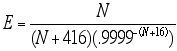
Now channel efficiency may be defined simply as the ratio of the number of bits in one frame as provided by the source, to the total number of bits transmitted in successfully communicating a frame. That is: the numerator is just “the message,” while the denominator takes into account the message, the overhead, the CRC, and the expected number of necessary retransmissions.
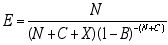
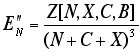
Thus the formula is:
,
where E = channel efficiency
N = frame length in bits
C = cyclic redundancy check length, in bits
X = overhead cost in bits
B = bit error rate .
 .
.
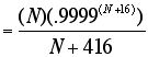
The graph does exhibit the predicted behavior: the value of E “peaks” for some positive value of N, a value that appears to be in the 1000 - 2500 range.
In order to apply numerical methods, we would prefer to find zeros, rather than maxima, of functions. Fortunately, we can transform this problem simply by applying an implication of the Mean Value Theorem: if E(N) has a maximum in an interval, then its derivative E’ (N) must have a zero. We have the option of:
1) differentiating E(N), the function graphed above, in which X, C, and B have already been assigned values. The disadvantage here is that in a new application with any of X, C, or B changed (e.g., a different transmitter), a new function would result and a new derivative would need to be calculated;
or
2) differentiating E(N,X,C,B) with respect to N. This partial derivative would be applicable as any parameter might be adjusted.
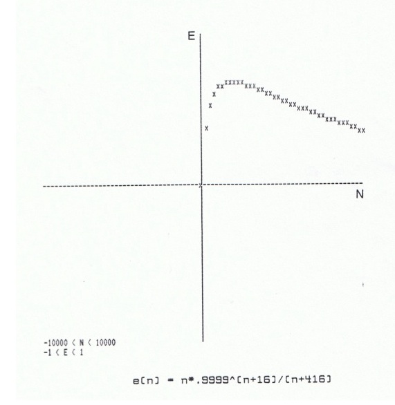
If we choose option 2), we have the partial derivative
 .
.
Let us examine the graph of this derivative function with the same values as before for X, C, and B:
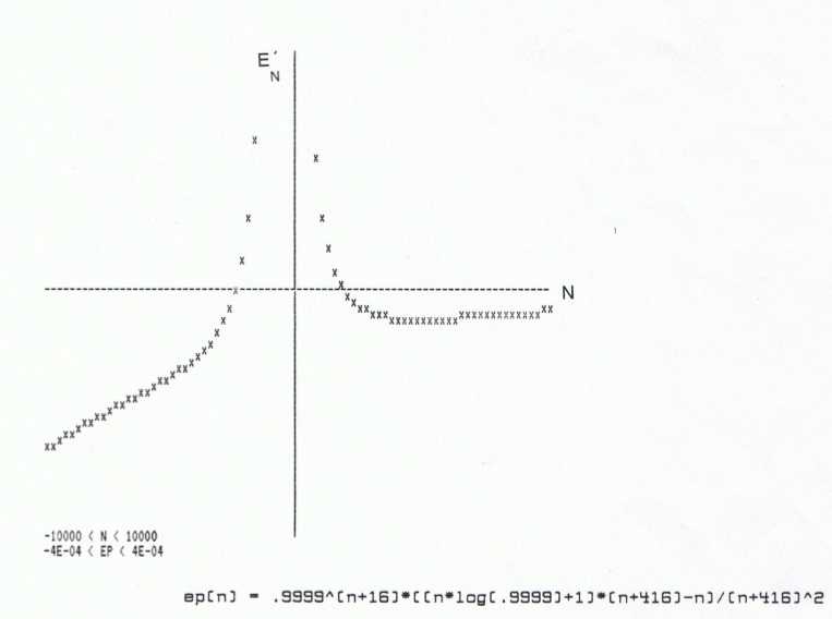
The graph does appear to cross the N-axis at a value of N for which the graph of the original function had a maximum. The task now is to determine the N-intercept with some precision, and we can use numerical methods to accomplish this.
Let us use the given typical values of X, C, and B, and use [1000, 2500] as our “candidate” interval for containing a zero of E'N . In all of the following calculations, let us require satisfaction of a residual-norm tolerance of 10-9; for those methods providing an interval of convergence, let us additionally require that an x-norm (actually, here, an “N-norm”) tolerance of 1* be satisfied.
* An uncharacteristically large x-norm tolerance is chosen because 1) N will eventually be converted to bytes (i.e., divided by 8) and rounded to an integer, so greater precision would be of little practical value; 2) with a BER rather imprecisely given as “10-4,” an x-norm tolerance even this small is rather presumptuous!
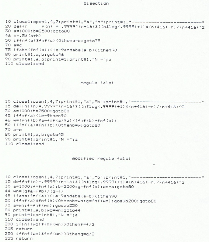
Here are the results of applying bisection:
a________________b
1000_____________2500
1750_____________2500
1750_____________2125
1750_____________1937.5
1750_____________1843.75
1796.875__________1843.75
1820.3125_________1843.75
1832.03125________1843.75
1837.89063________1843.75
1840.82031________1843.75
1840.82031________1842.28516
1841.55273________1842.28516
1841.91895________1842.28516
1842.10205________1842.28516
1842.10205________1842.1936
1842.10205________1842.14783
1842.12494________1842.14783
N = 1842.12494
regula falsi:
a________________b
1000_____________2500
1000_____________2217.98784
1000_____________2052.82173
1000_____________1958.84397
1000_____________1906.33323
1000_____________1877.30733
1000_____________1861.3619
1000_____________1852.63261
1000_____________1847.86295
1000_____________1845.25958
1000_____________1843.83944
1000_____________1843.06499
1000_____________1842.64273
1000_____________1842.41253
1000_____________1842.28703
1000_____________1842.21861
1000_____________1842.18132
1000_____________1842.16099
1000_____________1842.1499
1000_____________1842.14386
1000_____________1842.14057
1000_____________1842.13877
1000_____________1842.1378
1000_____________1842.13726
1000_____________1842.13697
1000_____________1842.13681
1000_____________1842.13673
1000_____________1842.13668
1000_____________1842.13665
1000_____________1842.13664
1000_____________1842.13663
1000_____________1842.13663
1000_____________1842.13662
1000_____________1842.13662
1000_____________1842.13662
1842.13662________1842.13662
N = 1842.13662
and modified regula falsi:
a________________b
1000_____________2500
1000_____________2217.98784
1000_____________2052.82173
1000_____________1880.26876
1000_____________1814.98133
1866.88395_____________1814.98133
1866.88395_____________1842.63492
1841.59827_____________1842.63492
1841.59827_____________1842.13682
1841.59827_____________1842.13662
1841.59827_____________1842.13662
1842.13662_____________1842.13662
N = 1842.13662
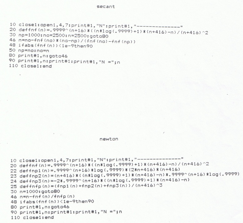
Applying the secant method, with N-1 = 1000 and N0 = 2500; tolerances as before, gives:
N
______________
2500
2217.98784
1625.40856
1903.41367
1851.7483
1841.69515
1842.13977
N = 1842.13977
The logical next step would be the Newton method. Newton requires the derivative of the function whose zero is sought: in this case, the second derivative of the original function E. If as before we choose to apply partial differentiation with respect to N, we obtain the following:
 ,
,
where 


After substituting numerical values for X, C, and B, we attempt Newton, with N0 = 1000, and with residual tolerance as before:
N
______________
1000
1417.89141
1723.17185
1831.99025
1842.06048
1842.13662
N = 1842.13662
Predictably, Newton, due to its quadratic convergence, requires the fewest steps -- at the cost of some complicated algebraic manipulation in determining  .
.
In all the above methods, the resulting N of approximately 1842 would be converted to the nearest integral number of bytes by the formula:
Number of bytes = int [N/8 + .5],
i.e., 230 bytes (= 1840 bits). This would be the actual optimum frame size. The value of E would be 0.6774, so the transmission of a message of K bits would require an overall expenditure of K/E, or 1.476 K, bits.
One might then explore the advantage of seeking a better channel (or perhaps the savings on equipment for a lower-quality channel!). This would involve fixing X and C as before, and trying different values for B. How is efficiency affected by using a channel with a BER of, say, 3 x 10⁻⁵ (i.e., about three times better than before)? Or ten times as good (BER = 10-5)?
Using values as before for X and C, the resulting values for N and 1/E, as these quantities vary with B, are shown:
BER..........Optimum # bytes.......1/E
10-3................59................3.066
3 x 10⁻⁴..........123................1.921
10-4................230................1.476 .
3 x 10⁻⁵...........440................1.243
10-5................781................1.136
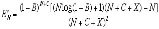
Here is a graph of 1/E (at optimum N) as a function of B:
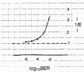
These were calculated using the secant method, tolerances as before.
Actual dollar costs would have to be considered in practice, but the above table and graph could be used for a rough guideline.
Results of the sort calculated here proved useful in the design and implementation of the data communication system described; the foregoing is an illustration of the power and practicality of numerical approximation methods.
References:
King, James G. Personal communications with the author: Letters dated 10/18/94 and 11/30/94; telephone conversation, 11/94.
The text of this paper (including formulae and equations) was produced on a Macintosh Performa 630CD computer with the aid of ClarisWorks 2.1 word processing, and printed in Helvetica font on a Hewlett Packard DeskWriter 540 printer.
All programs were run, and the first two graphs, all convergence sequences, and program listings were printed, using a Commodore 64 computer and a Star Micronics SG-10 printer.
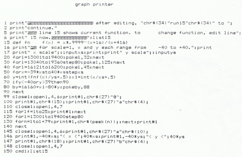
All programs (listings of which follow) were written in BASIC by the author. “Graph printer” was created circa 1990; all others in 1995.